[머신러닝] Linear Regression 1

04 Dec 2020

머신러닝

Linear Regression(수업방식)

간단한 예제를 통해 Linear Regression 을 알아본다.

1. Training Data Set

ML에 입력으로 사용될 데이터를 Numpy의 ndarray 형태로 준비한다.

import numpy as np
import matplotlib.pyplot as plt

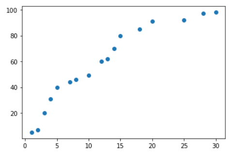
x_data = np.array([1,2,3,4,5,7,8,10,12,13,14,15,18,20,25,28,30]).reshape(-1,1)
t_data = np.array([5,7,20,31,40,44,46,49,60,62,70,80,85,91,92,97,98]).reshape(-1,1)

plt.scatter(x_data.ravel(),t_data.ravel())
plt.show()

2. Linear Regression model 정의

y = Wx + b 와 같이 Linear regression model( Hypothesis )을 정의한다. 여기서 W는 weight이고 b는 bias를 의미한다. 이 예제에서는 랜덤값을 사용한다.

W = np.random.rand(1,1)
b = np.random.rand(1)
## 주의해야 할 점은 W와 같은 경우 Multiple Linear Regression 고려해 nx1 꼴로 만들어주는게 효율적이다.

H = np.dot(x_data, W) + b

3. loss function 정의

loss function(손실함수)는 cost function 이라고도 불린다.

def loss_func(x, t):
    
    y = np.dot(x,W) + b  # y = XW + b
    return np.mean(np.power(t-y,2))  # 최소제곱법

4. Learning rate 정의

learning rate를 정의한다. 일반적으로 초기에는 1e-4 정도로 설정하고 loss 값을 확인하고 수치를 조절한다.

learning_rate = 1e-4

5. 학습 진행

Gradient Descent method를 이용해서 W와 b를 update 하는 방식으로 구현한다.

f = lambda x : loss_func(x_data, t_data)
for step in range(30000):
    
    W = W - learning_rate * numerical_derivative(f,W)
    b = b - learning_rate * numerical_derivative(f,b)
    
    if step % 3000 == 0 :
        print('W : {}, b : {}, loss : {}'.format(W,b,loss_func(x_data,t_data)))

W : [[0.27795254]], b : [0.46235041], loss : 3615.5725693594673
W : [[3.92221962]], b : [3.52920071], loss : 146.34608793662366
W : [[3.79606552]], b : [5.89354627], loss : 127.60313828483086
W : [[3.69227693]], b : [7.83872359], loss : 114.91685419386076
W : [[3.60688873]], b : [9.43904584], loss : 106.33006251890744
W : [[3.53663876]], b : [10.75565142], loss : 100.51803823028591
W : [[3.47884322]], b : [11.83883966], loss : 96.58413280783454
W : [[3.43129408]], b : [12.72999248], loss : 93.92144402605456
W : [[3.3921748]], b : [13.4631553], loss : 92.11918627268237
W : [[3.35999087]], b : [14.06633772], loss : 90.89931670632278

6. 예측

학습을 통해 얻어낸 W 와 b를 가지고 예측을 할 수 있다.

def predict(x):
    
    return np.dot(x,W) + b

print(predict(30))
## [[114.53841039]]

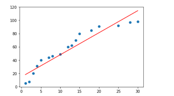
7. 그래프로 확인

학습을 통해 얻어낸 W 와 b를 가지고 직선 그래프를 그려본다.

plt.plot(x_data,np.dot(x_data,W)+b,'r')
plt.show()