[머신러닝] Decision Tree 3

04 Dec 2020

머신러닝

Linear Regression(sklearn)

` sklearn(사이킷런) 을 이용한 linear regression 방법에 대해서 알아본다. sklearn` 은 데이터분석, ML library 중 하나로 굉장히 유명하고 효율적인 library이다.

1. Raw Data Loading(raw 데이터 불러오기)

예제로써 온도에 따른 오존량을 추측하는 ML 시스템을 만든다. csv 파일로 된 데이터를 가져온다.

import numpy as np
import pandas as pd
import matplotlib.pyplot as plt
from sklearn import linear_model     # sklearn에서 linear_model을 불러온다.

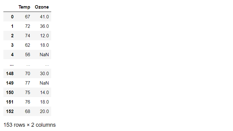
df = df.read_csv('./data/ozone.csv')
display(df)

training_data=df[['Temp','Ozone']]
display(training_data)

2. Data Preprocessing(데이터 전처리)

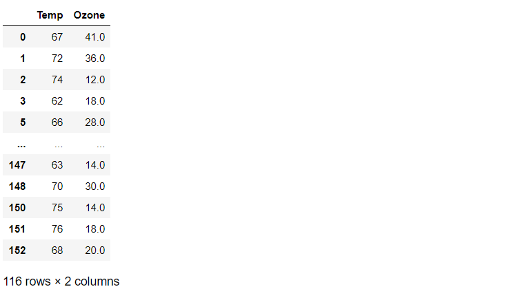
데이터를 다룰 때 여러가지의 전처리가 있지만 여기서는 결측치 제거만 한다.

training_data = training_data.dropna(how='any')
display(training_data)

3. Training Data Set

x_data와 t_data를 정의한다.

x_data = training_data['Temp'].values.reshape(-1,1)
t_data = training_data['Ozone'].values.reshape(-1,1)

4. linear regression model 객체 생성

sklearn을 활용해 학습되지 않은 linear regression model 객체를 생성한다.

model = linear_model.LinearRegression()

5. Training Data Set을 이용해서 학습 진행

fit method를 이용해서 학습을 진행한다.

model.fit(x_data, t_data)

6. W와 b 값을 알아내기

weight는 ceef_, bias는 intercept_ 라는 명령어로 알아 낼 수 있다.

W = model.coef_
b = model.intercept_
print('W : {}, b : {}'.format(W,b))
## W : [[2.4287033]], b : [-146.99549097]

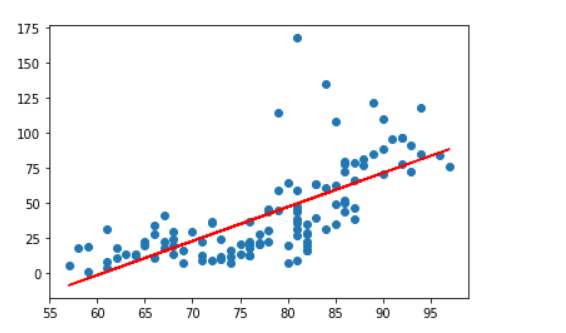
7. 그래프로 확인

plt.scatter(x_data, t_data)
plt.plot(x_data, np.dot(x_data,W) + b , color='r')
plt.show()

8. 예측

predict_val = model.predict([[80]])  # 이중 list가 아니면 error
print(predict_val)  
## [[47.30077342]]

알아야 할 keyword

model = linear_model.LinearRegression, model.fit, model.coef_, model.intercept_, model.predict