[머신러닝] Decision Tree 4

04 Dec 2020

머신러닝

Linear regression (tensorflow)

tensorflow를 이용한 아주 간단한 linear regression 방법에 대해서 알아본다.

다음의 `Training Data set을 보자.

x_data = [1, 2, 3, 4, 5]
t_data = [2, 4, 6, 8, 10]

1. placeholder 만들기

placeholder를 사용해서 프로그래밍한다. placeholder를 만들때는 shape 과 dtype을 명시해 주지만 1차원인 경우 shape을 명시하지 않아도 된다.

import tensorflow as tf

X = tf.placeholder(dtype = tf.float32) 
T = tf.placeholder(dtype = tf.float32)

2. weight & bias 초기값 설정

정규분포의 random값을 이용해 초기값을 설정한다.

W = tf.Variable(tf.random.normal([1]), name ='weight')
b = tf.Variable(tf.random.normal([1]), name ='bias')

값이 바뀔 수 있는 경우 tf.constant 가 아닌 tf.Variable이 사용된다.
name은 tensorflow 내부적으로 사용되기 때문에 입력해준다.

3. Simple Linear Regression Model(Hypothesis)

Simple Linear Regression Model 을 설정해 준다.

H = W * X + b

4. Loss function 정의

Loss function을 정의한다.

loss = tf.reduce_mean(tf.square(H-T))

tf.reduce_mean : 각 원소마다 제곱해주는 함수이다.
tf.square : 모든 원소들을 평균내준다.

5. Train node 생성

forloop에서 사용될 train node를 생성한다. Gradient Descent method를 사용할것이다.

train = tf.train.GradientDescentOptimizer(learning_rate=1e-4).minimize(loss)

tf.train.GradientDescentOptimizer : gradient descent optimizer를 사용한다.
learning_rate : 1e-4 값을 사용하고 수정가능하다.
minimize(loss) : 어떤것을 minimize 할지 결정해준다.

6. Session 생성 및 초기화

tensorflow 1.x 버전에서는 session을 생성하고 초기화 해주는 단계가 필요하다.

sess = tf.Session()
sess.run(tf.global_variables_initializer())

7. 학습 진행

forloop 를 이용해 학습을 이용해 준다.

for step in range(30000):
    _, W_val, b_val, loss_vale = sess.run([train, W, b, loss], feed_dict={X:x_data, T:t_data})
    
    if step%3000==0:
        print('W : {}, b : {}, loss : {}'.format(W_val, b_val, loss_val))
        
## W : [0.9734955], b: [-0.5662528], loss : 15.472111701965332
## W : [2.064629], b: [-0.2368326], loss : 0.010198862291872501
## W : [2.0592186], b: [-0.21375798], loss : 0.008317629806697369
## W : [2.053498], b: [-0.19317965], loss : 0.006792913191020489
## W : [2.0483887], b: [-0.17459047], loss : 0.005549082066863775
## W : [2.0437307], b: [-0.15776387], loss : 0.004531101323664188
## W : [2.0394826], b: [-0.14258331], loss : 0.0037005171179771423
## W : [2.0357387], b: [-0.12886304], loss : 0.003023307304829359
## W : [2.032248], b: [-0.11645487], loss : 0.002468559192493558
## W : [2.0291922], b: [-0.10525043], loss : 0.0020168586634099483

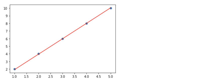
8 . 그래프를 통해 확인

그래프를 확인해 간단히 확인해 본다.

import matplotlib.pyplot as plt

plt.scatter(x_data, t_data)
plt.plot(x_data, W_val*x_data+b_val, color='r')
plt.show()