[머신러닝] Logistic Regression 1

04 Dec 2020

머신러닝

Logistic Regression 쉬운 예제(1)(python구현)

Logistic Regression의 쉬운 예제를 통해 구현을 해본다.

Training Data Set

공부시간과 합격에 관한 아주 작은 Data Set을 만든다.

시간	2	4	6	8	10	12	14	16	18	20
합격여부	0	0	0	0	0	0	1	1	1	1

Python code

numpy와 pandas를 이용해 구현한다.

0. 수치미분

import numpy as np

def numerical_derivative(f,x):

    h = 1e-4
    derivative_x = np.zeros_like(x) # 미분한 결과를 저장하는 ndarray
    
    # iterator를 입력변수 x에 대해 편미분을 수행
    it = np.nditer(x, flags=['multi_index'])
    
    while not it.finished:
        
        idx = it.multi_index  
        
        tmp =x[idx]
        
        x[idx] = tmp + h
        fx_plus_h = f(x)   # f(x + h)
        
        x[idx] = tmp - h
        fx_minus_h = f(x)  # f(x - h)
        derivative_x[idx] = (fx_plus_h - fx_minus_h)/(2*h)
        
        x[idx] = tmp
        it.iternext()
    return derivative_x

1. Training data 및 Library

import numpy as np
import pandas as pd

x_data = np.arange(2, 21, 2).reshape(-1,1)
t_data = np.array([0,0,0,0,0,0,1,1,1,1]).reshape(-1,1)

2. Weight 및 Bias

input_var = np.random.rand(2,1) # W, b 모두 포함하게 만든다.

3. Loss Function

def loss(input_var):
    A = np.concatenate([x_data, np.ones_like(x_data), axis=1)
    z = np.dot(A,input_var)
    y = 1/(1+np.exp(-z))
    
    delta = 1e-7 # 로그 연산시 무한대로 발산하는것을 방지한다.
    
    # cross entropy
    return -np.sum( t_data*np.log(y+delta) + (1-t_data)*np.log(1-y+delta)) 

4. Learning process

learning_rate = 1e-4
for step in range(30000):
    input_var -= learning_rate*numerical_derivative(loss, input_var)
    
    if stage%3000 == 0:
        print('W : {}, b : {}, loss : {}'.format(input_var[0],input_var[1], loss(input_var)))

## 결과
W : [0.98832513], b:[0.54972081], loss : 44.869531753345434
W : [0.04402015], b:[-0.13461262], loss : 6.453814777928654
W : [0.08159956], b:[-0.64914488], loss : 5.564879557034531
W : [0.1141694], b:[-1.09157614], loss : 4.9077073635929995
W : [0.14261162], b:[-1.47609988], loss : 4.411418723694001
W : [0.16771556], b:[-1.8145136], loss : 4.027108596702506
W : [0.19012277], b:[-2.11603215], loss : 3.722091077583651
W : [0.21033534], b:[-2.38770113], loss : 3.47451776539932
W : [0.22874206], b:[-2.6348987], loss : 3.2695649058908196
W : [0.2456447], b:[-2.86176157], loss : 3.096962629227913

5. Prediction

def logistic_predict(x)
    A = np.concatenate([x, np.ones_like(x)],axis=1)
    y = A * input_var  # y= wx+b
    Z = 1/(1+np.exp(-y)) 
	
    if z >= 0.5:
        result = 1
    else:
        result = 0

    return z, result

study_hour = np.array([[13]])
result = logistic_predict(study_hour)
print('공부시간 : {}, 결과 : {}'.format(study_hour,result))

######### python 결과값 ##########
공부시간 : [[13]], 결과 : (array([[0.58057319]]), 1)

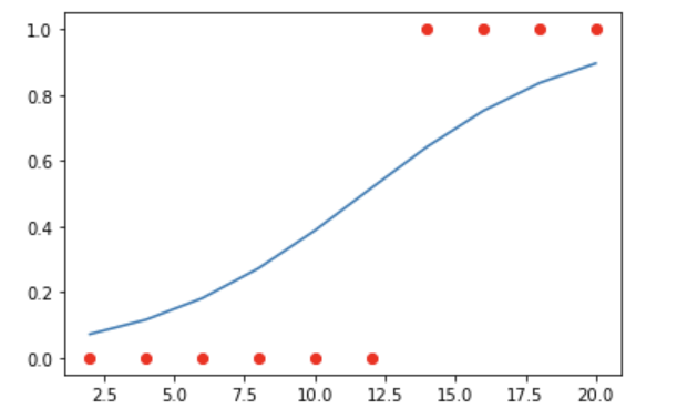
6. 그림으로 확인

import matplotlib.pyplot as plt
A = np.concatenate([x_data, np.ones_like(x_data)],axis=1)
z = np.dot(A,input_var)
y = 1/(1+np.exp(-z))
plt.plot(x_data, y)
plt.scatter(x_data, t_data, color='red')
plt.show()