[머신러닝] Decision Tree 2
Decision Tree(예제)
독립변수가 여러개 있을 때 선택 방법과
sklearn을 통해 간단히 구현해본다.
독립변수 여러개 있을 때 분기방법
날씨에 다른 경기 여부에 대한 다음 표를 통해 분기방법에 대해서 알아본다.

위의 표를 보면 OUTLOOK, HUMIDITY, WIND 의 3가지의 독립변수와 PLAY 라는 종속 변수가 하나 있다.
-
우선 분기 되지 않았을때의 entorpy의 계산한다.
YES: 9,NO: 5import numpy as np print(-(9/14)*np.log2(9/14)-(5/14)*np.log2(5/14)) # 0.9402859586706311 -
각 독립변수 기준으로 분기되었을때의 entropy를 계산한다.
-
OUTLOOK:SUNNY(YES: 2NO: 3 ),OVERCAST(YES: 4NO: 0),RAIN(YES: 3NO: 2)print((5/14)*(-(3/5)*np.log2(3/5)-(2/5)*np.log2(2/5))\ + (4/14)*(-4/4*np.log2(1))\ +(5/14)*(-(2/5)*np.log2(2/5)-(3/5)*np.log2(3/5))) # 0.6935361388961918 # 정보 획득량 : 0.24674981977443933 -
HUMIDITY:HIGH(YES: 3NO: 4 ),NORMAL(YES: 6NO: 1 )print((7/14)*(-(4/7)*np.log2(4/7)-(3/7)*np.log2(3/7))\ +(7/14)*(-(1/7)*np.log2(1/7)-(6/7)*np.log2(6/7))) # 0.7884504573082896 # 정보 획득량 : 0.15183550136234159 -
WIND:WEAK(YES: 6NO: 2 ),STRONG(YES:3NO:3)print(-(8/14)*((2/8)*np.log2(2/8) +(6/8)*np.log2(6/8))\ -(6/14)*((3/6)*np.log2(3/6) + (3/6)*np.log2(3/6))) # 0.8921589282623617 # 정보 획득량 : 0.04812703040826949 -
결론 : 정복 획득량이 가장 많은 OUTLOOK 을 기준으로 분기해야 한다.
BMI 예제
mlxtend.plotting의plot_decision_regions을 통해 분할 영역을 초점을 맞쳐 살펴본다.
import numpy as np
import pandas as pd
import matplotlib.pyplot as plt
from sklearn.tree import DecisionTreeClassifier
from mlxtend.plotting import plot_decision_regions # machine learning extend
## training data set
df= pd.read_csv('./data/bmi.csv', skiprows=3)
x_data = df[['height', 'weight']].values
t_data = df['label'].values
num_of_sample = 100
x_data_red = x_data[t_data==0][:num_of_sample]
t_data_red = t_data[t_data==0][:num_of_sample]
x_data_blue = x_data[t_data==1][:num_of_sample]
t_data_blue = t_data[t_data==1][:num_of_sample]
x_data_green = x_data[t_data==2][:num_of_sample]
t_data_green = t_data[t_data==2][:num_of_sample]
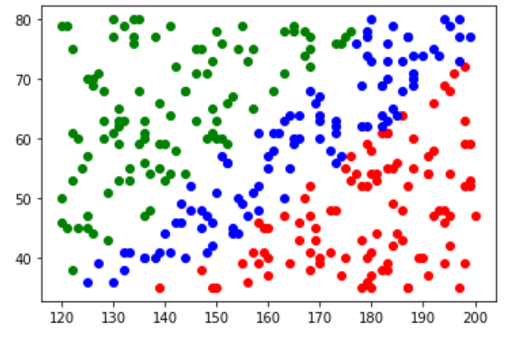
plt.scatter(x_data_red[:,0],x_data_red[:,1], color='r')
plt.scatter(x_data_green[:,0],x_data_green[:,1], color='g')
plt.scatter(x_data_blue[:,0],x_data_blue[:,1], color='b')
plt.show()
x_data_sample = np.concatenate((x_data_red, x_data_blue, x_data_green), axis=0)
t_data_sample = np.concatenate((t_data_red, t_data_blue, t_data_green), axis=0)

model = DecisionTreeClassifier()
model.fit(x_data_sample, t_data_sample)

plot_decision_regions(X = x_data_sample, y= t_data_sample, clf=model, legend=2)
plt.show()
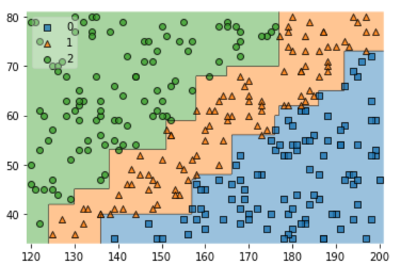
- 분류하는데 있어서 SVM 과 확실한 차이를 볼 수 있다.
MNIST 예제
독립변수가 이산값이지만 너무 많아서 continuous 한 값에 가까운 예제에 대해서 accuracy를 살펴보는것을 목표로 한다.
import numpy as np
import pandas as pd
from sklearn.tree import DecisionTreeClassifier

from sklearn.preprocessing import MinMaxScaler
from sklearn.model_selection import train_test_split
from sklearn.metrics import classification_report

df = pd.read_csv('./data/mnist/train.csv')

## Data Split
x_data_train, x_data_test, t_data_train, t_data_test = \
train_test_split(df.drop('label', axis=1, inplace=False), df['label'], test_size=0.3, random_state=0)
## Min-Max Normalization
scaler = MinMaxScaler()
scaler.fit(x_data_train)
x_data_train_norm = scaler.transform(x_data_train)
x_data_test_norm = scaler.transform(x_data_test)

del x_data_train
del x_data_test

model = DecisionTreeClassifier()
model.fit(x_data_train_norm, t_data_train)

result = model.predict(x_data_test_norm)
print(classification_report(t_data_test, result))
##               precision    recall  f1-score   support
##
##            0       0.90      0.91      0.91      1242
##            1       0.93      0.95      0.94      1429
##            2       0.83      0.79      0.81      1276
##            3       0.80      0.81      0.81      1298
##            4       0.85      0.85      0.85      1236
##            5       0.78      0.80      0.79      1119
##            6       0.88      0.89      0.89      1243
##            7       0.89      0.87      0.88      1334
##            8       0.80      0.76      0.78      1204
##            9       0.80      0.83      0.81      1219
##
##     accuracy                           0.85     12600
##    macro avg       0.85      0.85      0.85     12600
## weighted avg       0.85      0.85      0.85     12600
- 정확도가 다른 classifier에 비해 낮은것을 알 수 있다. 이유는 yes/no 와 같이 이분적이기 보다 결과 값이 너무 많기 때문이다.